The SA broadband antenna system has much in common with the SDR shown below it in the block diagram. Both of these have major differences when compared to older, conventional analog receive system types. Unlike analog receivers, each of these is fundamentally very broadband. Rather than filtering in frequency to separate incoming signals prior and during amplification, these systems accept a very broad frequency spectrum and sample the unfiltered aggregate. Selectivity is created within the DSP processes that follow the hardware and which are inherent in any SDR.
Because there isn't selectivity within the range to be received, all of the components and circuits have a unique challenge - they must simultaneously tolerate the instantaneous aggregate of all input signals present while also providing the ability to process very weak signals. They must have very high dynamic range.
Unlike older analog receive system architectures, when these attributes aren't provided, when the instantaneous total of all signals impinging on the system exceeds some maximum, failure occurs. Also unlike previous analog receivers, this failure tends to occur suddenly rather than gradually. When an analog receiver experiences overload it tends to generate intermodulation distortion (IMD) which creates unwanted signals and noise. When a broadband, probe type receive system experiences too high input level from all signals within the entire spectrum it ceases to function almost instantly. That temporary failure may occur at stages within the active antenna system portion or, if the overload first occurs within the SDR, at that LNA preamplifier. It can also happen if the maximum tolerable ADC level is exceeded.
The characteristics of signal overload are so different and the consequences so much greater and more immediate that they need to be understood and recognized when they occur because the entire system becomes unusable for the duration of the overload. Because overloading occurs as the instantaneous vector sum of all signals over the entire broad bandwidth of the system it may not be persistent. As an example if there are many MW AM broadcast band signals simultaneously modulating, the instantaneous modulation peaks of all these different contents together may be very much greater than the carrier magnitude of any one of them alone. Even if there are only two equal size large signals having 100% modulation the instantaneous peak power may be 12 dB greater than the carrier power of either alone. If there are many such signals overloading may occur when the individual carriers are each lower than this. This forces a requirement of sufficient "headroom" on a these systems.
Also, for the High-Z broadband probe/SDR option, out-of-band signals which are not even visible in a display may contribute to overloading. Even if a system is only being used to operate over, say, 0-30 MHz large FM broadcast signals in the 100 MHz region may overdrive the SAS input buffer stages and generate distortion products.
The deployment environment may determine whether the High-Z or Medium-Z option of the SAPreamp is necessary. For very strong signal environments, it may not be possible to operate a VLF-VHF SAS and the sacrifice of VLF operation may have to made.
In summary, because these broadband systems are so different from previous receivers which used tuned/matched antennas and analog filtering for selectivity, to prevent overload that manifests differently it is essential to understand and recognize the failure modes and eliminate them in order for the system to operate properly.
The symptoms of overload in the SAS can be more difficult to recognize. In most environments , overly strong signals at the antenna terminals, often from very large AM BCB transmitters near 1 MHz or FM BCB transmitters near 100 MHz, cause the input buffer OpAmp stage to produce unwanted noise and/or mixing products. The ADA4930 stages have impressively good distortion performance so at least with typical stage gain settings as used in the SAS reference design, these do not contribute to the unwanted degradation in the SAS output. Because the aggregate signal at the terminals can be very complex and because it can vary from situation to situation, learning the characteristics of the buffer distortion artifacts is important.
Also, because the largest signals impinging on the SAS may not be in the operating range of an SDR which follows, it may not be easy to recognize that a degradation is due to overload at the antenna input.
As an example, the spectral plots below demonstrate two types of site noise. One type is a generally flat and unfeatured broadband noise floor with little variation. This is characteristic of the noise described by the ITU measurements. In this example, that level is between "Quiet Rural" and "Rural". It is characteristic of noise from a very large number of sources with no single source being obvious.
Also evident are some more complex shapes that are not from noise of the type described by the ITU. Instead, these regions - 5MHz to 10 MHz for example - show structure that is attributable to local, probably near-field, noise ingress. While careful positioning of the SA might reduce this structured noise, it probably will have little or no effect on the wider, flatter noise will be a limit for that site and nearby regions as a whole.
Changes to shaping which do not increase the SA noise floor above the broadband, flatter noise will likely not affect recovered SNR since it is being set by the general region. If a large signal that drives the SA preamp into visible distortion is present then simply decreasing the dipole length may be sufficient. In this particular example, a 60 kHz transmission from the 20km distant 110kW transmitter of WWVB is producing an output signal above -10 dBm. This large signal aggregating with multiple large AM BCB signals occasionally pushes some part of the system, either the SA preamp or the SDR that follows, into distortion which causes noise floor lift across the entire spectrum. Here only a slight decrease in the value of Rp might be very beneficial.
Each situation will require analysis of signal levels during day, season and even over a solar cycle to determine optimum adjustments. A general solution for the adjustments is beyond the scope of this article. Don't forgot to look above the range visible on the SDR since the SA preamp generally has flat response beyond 200 MHz. A large local VHF or UHF signal may be causing or exacerbating overload yet be unseen.
Here is a spectrogram obtained using a KiwiSDR showing the results of occasional overloading peaks in the receive system.
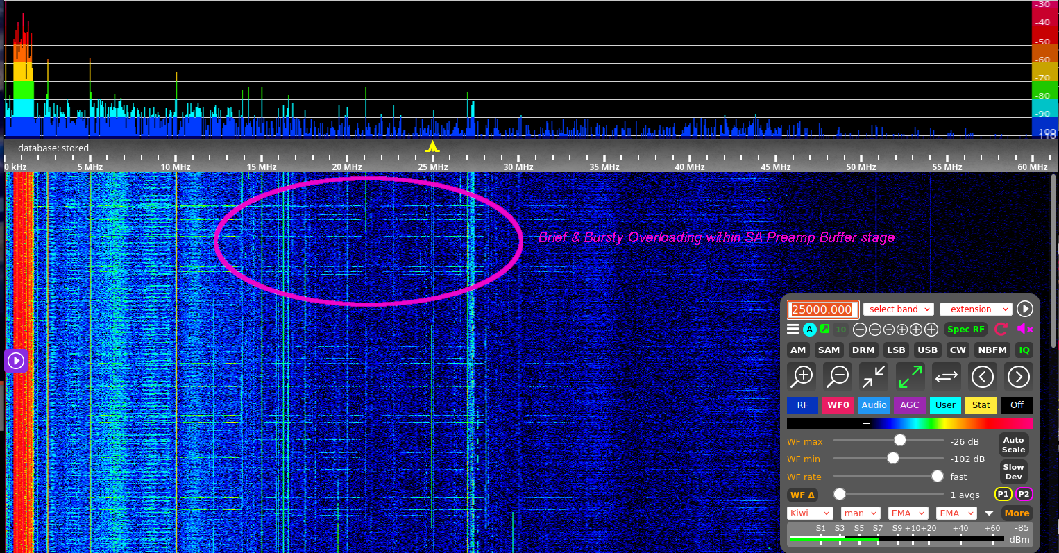
Short term sporadic lines across the spectrum from these kinds of overload are most easily seen on wide frequency display such as WebSDR as is used on a KiwiSDR or Web-888 by selecting a broad span with spectral and waterfall averaging set to 1 - to no averaging at all. Because they are brief and sporadic, averaging tends to make them difficult to recognize. Notice that these generate components above the MUF which is an indication that they are locally created rather than over-the-air.
These events can occur when the instantaneous sum of all signals becomes large enough to either over-run the ADC within the SDR or create distortion within the SA preamp, or both. When they occur they may exhibit in a manner similar to broadband impulse noise such as lightning. This may be coincident with an observable change in amplitude of existing signals. Overloading may be due to or exacerbated by large out-of-band signals such as FM broadcast near 100 MHz. Study and testing is necessary to determine which is the cause in order to determine a best solution.
In this example the problem was more extreme when a 6m dipole was used but much less troublesome when antenna length was only reduced to 5m. This is the case because the signal levels are from local rather than ionospheric sources so are very stable in amplitude. If the overload had involved HF ionospheric signals this would probably not have been the case.
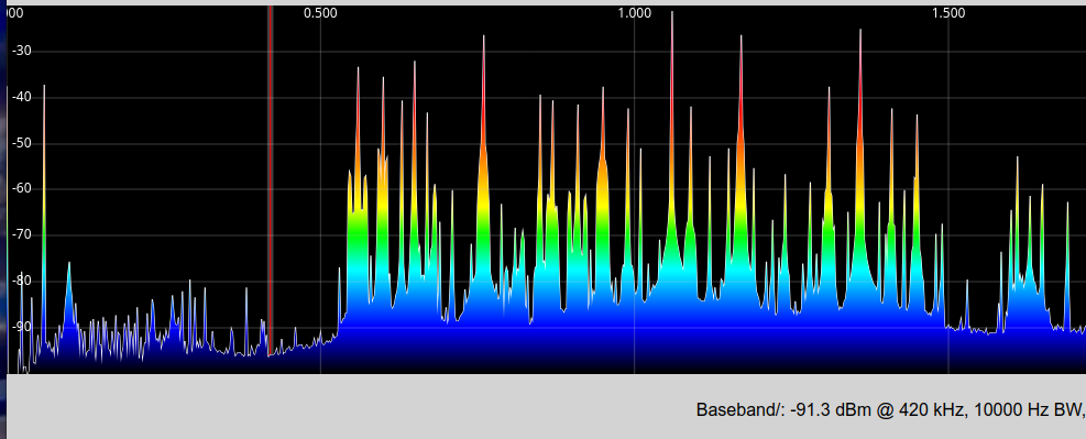
More severe overload of the input buffers of the SAS will be indicated by a ShackBoard output voltage much above 600 mV peak-peak. Particularly in environments with large MW/AM BCB signals, it can be useful to compare the SNR between one of these large signals with the noise floor just below that band, perhaps near 475 kHz. In a system that is not in overload particularly during the daylight hours when absorption is high there will generally be a very high SNR. The following image shows an example of a healthy system:
[A special comment to anyone having particular difficulty keeping the input high impedance buffers from overloading even with value changes and contemplating major design change:]
When overload occurs in this stage, the symptom is generally as shown above. The mechanism of overload and nonlinearity that will be observed is usually that of a tendency toward oscillation during the signal peaks. This happens when the slew rate capability of the ADA4817 OpAmp is insufficient for the high signal level and thereby creates an extra pole in the open loop response with the attendant extra phase shift. In this situation the circuit is no longer stable and oscillation occurs. It may be useful to recognize this if significant design change is contemplated.
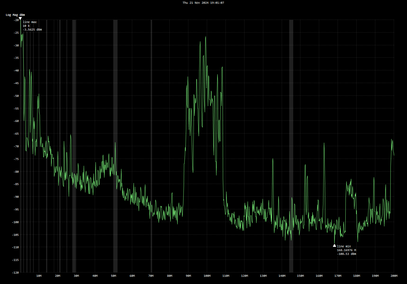
The following 10 kHz to 200 MHz spectrogram was taken soon after local sunset in Fort Collins, Colorado using a TinySA-Ultra with RBW=300 kHz to capture the output from a 5m SA system having an older CAT driver with gain set to 14 dB - a previous setting which is a bit high of what may be a desirable for general purpose use. Approximately 30m of CAT5 cable is between the SA Preamp and the Shack Board. The Shack Board being used had 0 dB gain.
This plot also demonstrates the ability of the SA system to operate at VHF. While there are many signals below 30 MHz, except for nearby 110 kW WWVB at 60 kHz, the FM broadcast stations near 100 MHz are the strongest signals over the entire range. The large amplitude of these is partially because they are largely line-of-sight and transmitting high power .They are probably contributing significantly to the peak instantaneous amplitude. Because they are higher frequency they also demand higher slew rate and large signal performance from the input buffer OpAmps. These may not be directly detrimental at the SDR that is used if it has a lowpass filter as most do but since all of these signals are present at the SA Preamp they do contribute to maximum instantaneous signal and may cause overload in either the high impedance buffer stage or the CAT cable driver there and before the aggregate signal reaches an SDR. As a c heck, the strongest FM BCB signal is measured to be -32 dBm on a nearby 75MHz - 2000 MHz Biconical indicating that even with CAT5 cable loss the overall SA system may still have 14dB - 9dB = 5 dB of gain as expected.
Antenna size together with R/C filtering before the input buffer amplifiers are used as a means of preventing overdrive in common use cases where AM and SW broadcast stations may produce very large field strength at the antenna that would otherwise drive the system into distortion and non-linear operation.
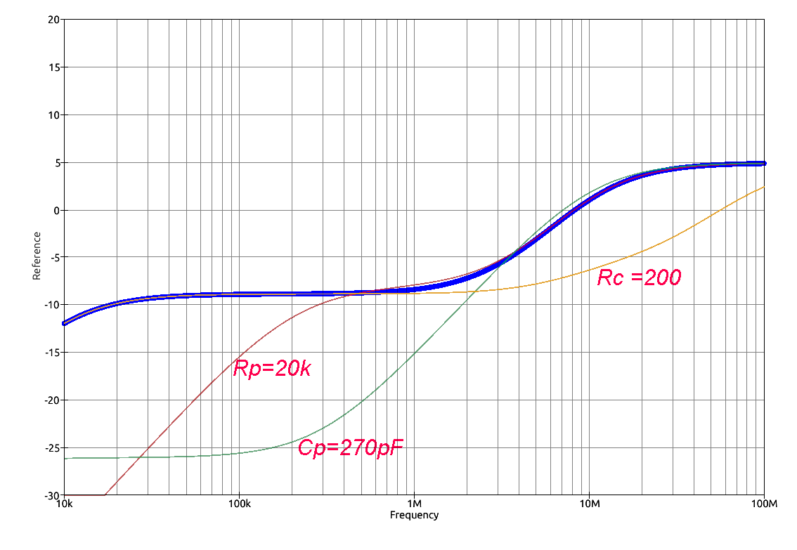
Adjusting antenna size or the RC/R shaping in the input buffers allows a degree of level adjustment and of pre-filtering to reduce the potential for overload. Traditional LC filters cannot be easily created with such high impedance antenna connections and wide bandwidths. Only R and C elements are used in the SAS for that reason. Depending upon the magnitude and frequency of an offending local signal, different courses of action may be indicated.

With the reference values shown, 6m antenna, Rc=2k, Rp=2M, Cp=33pF and G=2 the overall response should look approximately like this:
Usually adjustments will be made after identifying the portion of the spectrum that needs to be adjusted. Very generally these adjustments affect different regions:
If the degree of overload and its frequency can be identified, possible ways to reduce the level to take a system out of overload without compromising sensitivity at other frequencies may be understood in what follows.
To demonstrate the effect of changes, the following plots show the
Additionally simply shortening the dipole from 6m to 3m can reduce levels across the entire spectrum about -6 dB but potentially with a consequential degradation of the overall noise floor if unwanted ingress becomes significant at the lower levels. This might seem drastic but in regions such as "Residential" or "City" where the limiting broadband noise floor is significantly higher than "Quiet Rural", there may be a lot of unreachable headroom. Raising the SA noise floor and reducing the sensitivity may not have any significant adverse effect on the SNR of recovered signals.
All of these values are interactive so a Model and simulator such as QUCS-S:qucsator or Spice is useful in selecting them once a particular target result is known.
In general, sites with very low ITU broadband regional noise, say Quiet Rural, but also near to sources of very strong signals, especially VHF ones, are the most difficult to optimize for dynamic range. Fundamental limitations of even the best components and designs can be seriously challenged to achieve the best results in situations of this sort.