Cloth Simulation

1. Abstract

Our final project consisted of 2 parts.

We studied the current literature on representing and rendering cloth in general, both statically, as well as dynamically (cloth animation). Consequently, we took upon implementing a particular algorithm for cloth representations, initiated and described by Jerry Weil in a 1986 SigGraph Paper.

We wrote a projective renderer from scratch, implementing many of the elements discussed during the course, but never covered by the assignments (such as soft shadows, integrated antialiasing, a better lighting model, extended texture mapping etc.)

The primary reason for submitting this paper in addition to the project is to describe both our new results and the unexpected difficulties we've encountered while working on cloth representation. Though we did start by following Weils paper, we radically diverged from it towards the end and instead devised a unique representation of our own which is better suited for projective rendering. Similarly, while working on the shadow algorithm, we added a few enhancements, which we felt were of peculiar interest and could be developed further.
Though we include relevant images in the actual body of the paper, we urge you to consider looking at the other, higher resolution pictures submitted with the project to get a better feel for what we did.

2. The Cloth Simulation : Weil's Algorithm

Our project takes advantages of previous results in the field of cloth representation. Specifically, the catenary was initially used by Weil to physically simulate the threads in a cloth.
A general catenary is described by the equation:

This equation describes the "path" that's taken by a thread when left hanging between two constraint points. The derivation is not interesting and/or relevant to the paper; should the reader want to investigate it more, we suggest reading a chapter on Calculus of Variations.
One important detail is that given a length and two constraint points, there is one unique catenary which describes that particular thread.

Another interesting result is that a catenary is self-similar, i.e., splitting a catenary into two parts will yield two catenaries. This property is used in our own cloth algorithms.

We started by perusing [WEIL86] on The Synthesis of Cloth Objects. The main idea behind the paper is a three step processing of the cloth material :

In the first step involves a mathematical approximation of the cloth using catenaries.

The second step involves a gradual relaxation of the cloth, using a simplified gravitational model (which, among other things, does not account for gravity)

The third and final step consists of representing the cloth with polygons once its lattice points have been relaxed and placed in their final positions.

Though apparently simple (at least, we thought so), the mathematical approximation of the cloth is extremely involved. We began by implementing the first step in Weil's algorithm. However, the literature was extremely vague and omitted some critical discussions on how to solve certain equations. Hence, we devised our own schema described below.

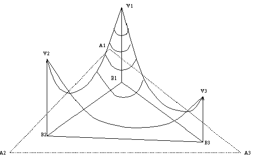
We start with 2 sets of 4 (three dimensional points). The first set (henceforth referred to as the set A) represents the 4 points that describe the extents of the cloth at rest (for instance, spread upon a flat surface). All these points are assumed to be, without loss of generality, in a plane, with 0 y-coordinate. The second set (henceforth referred to as the set B) represents the 4 points that describe the corners of the cloth when lifted in the air. At this stage, the problem is reduced to representing the threads of the cloth as they would fall naturally in between the points B, given that we know where the threads came from (the point lattice determined by A).

Pick a pair of opposite corners.

Draw the catenary between them.

Pick the other pair of opposite corners (the cloth is assumed to be rectangular) and find the catenary between them.

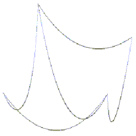
Since a point on a catenary can not fall any lower then the higher of the two catenaries without extra extension, Weil noted that it is admissible to entirely ignore the "lower" of two intersecting catenaries. The lower catenary is chosen by evaluating the y-value of each catenary at the point where their respective domains intersect. The domain of a catenary is simply the projection of the catenary curve on the x-z plane. It turns out that this domain is simply the straight line between point C1 and C2.

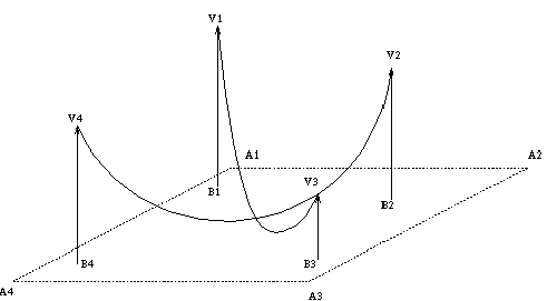
[In this image - the dotted lines represent the constraints of the relaxed cloth; the upward arrows represent the points of the B lattice and the curved lines are the catenaries between the B points]
Once the higher catenary is determined, two catenary triangles are formed, each of which shares the newly formed catenary as the hypotenuse.

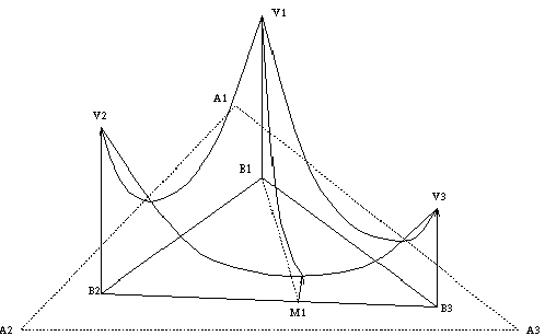
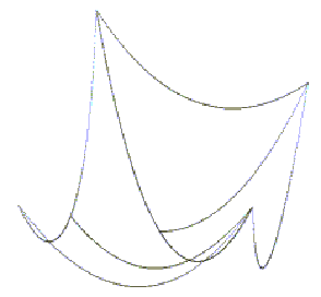
Iterate the following algorithm for as long as necessary :

Consider the 3 medians of each triangle such formed. The start and end point of the median can (easily) be determined in the B lattice. By a simple interpolation, we can also compute their origination in the in A lattice.

Each median becomes the domain of a new catenary. At this point, these three new catenaries split the triangle from which they originate.

Pick the highest catenary (in the same fashion as before) and split the triangle into two smaller triangles and repeat.

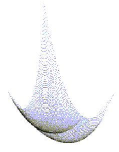
Here are some more images rendered with Weil's Division algorithm.

3. Detail on Weil's Algorithm

Another detail neglected in the original paper was a method to determine the medians and the lengths of the respective threads. We provide our particular algorithm for doing so:
Consider a triangle, T, with vertices V1, V2, V3 in the B lattice and corresponding vertices, A1, A2, A3 in A. Since the derivation for each median in particular is identical, we only present it for the median from V1 to the middle of (V2, V3). We know that the median has been issued at vertex V1 and goes to some point on the catenary between V2 and V3 (right "above" M1 - the middle of the segment (V2,V3). The difficult problem is determining the length of the thread between these 2 points in the original cloth, i.e., the A lattice.

If we ignore the elasticity of string, then we know that the length of the thread between (V2,V3) is the same as the Euclidean distance between A2,A3. However, we need to compute the length of the thread between V1 and the upward projection of M1 on the catenary C(V2,V3). The projection involves no more than evaluating the catenary equation at the point M1. Let M1 in C(V2,V3) be this projection. The computation of the thread length requires some cleverness. Suppose we could compute the thread length from V3 to M1. Let this length be . Since V3 corresponds to A3, we can conclude that the length of the thread we are looking for is the distance between A1 and the point situated at a distance , from A3 on the segment (A2,A3).
The computation of is no more than a simple integral :

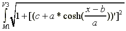
(where the squared term inside is the first derivative of the equation of the catenary between V2 and V3). The integral computes the length of the catenary curve in between the supplied domain points. Surely, the reader will realize that the integral bounds are stylized (the points are 2 dimensional - V3 and M1 - while the function is clearly 1 dimensional. What we mean here is to find the position of M1 on the line between V3 and V2, by a simple ratio computation).

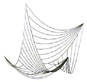
The subdivision process goes on until the user determines that sufficient accuracy has been obtained. We pushed it further up to 5 levels of subdivision (the last of which consisted of 40,000 B-lattice points). Here are a few images we produced using Weil's algorithm (the levels represented are 0, 1, and 4 respectively).

4. Elasticity problems

Ignoring the elasticity does contribute to error in the simulation. The other papers, e.g. Terzopulous, that have dealt with elasticity all require the solution of partial derivative equations arrived at through the physics of elasticity theory.
One of the most frustrating topics not covered in the paper was the computation of the equations of the catenaries between the threads. Here is a little input on what we came up on the subject :

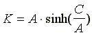
Should you choose to read the derivation provided by Weil at the end of his paper, you will realize that one of the first steps of the derivation consists of finding the solution of a transcendental equation:

The author correctly suggests that we try to find the solution of this equation by means of approximation. Hence, we attempted to find the solution by means of using the Newton-Raphson approximation. Although accurate, the errors inherently introduced in the computation propagate up to a level where the computation becomes impossible. For example, some of the results we were getting at division level 5 revealed that the length of the catenary between 2 legitimate points was shorter than the actual Euclidean distance between the points-a grotesque situation.
In order to solve this problem, we artificially elongated the length of the thread (computed by means of the line integral above) at every step until the thread was able to fit between the constraints. The heuristic we decided to use involved multiplying the length of the thread by a percentage of itself every step of the way until the equation was solvable. This way, we would successfully avoid a situation in which the thread barely fit between the points and looked like a straight line.

Unfortunately, while this enhancement allowed us to solve the first part of the derivation, problems ensued in the second part, where the new length of the thread fell outside the asymptotic boundaries of sinh and cosh (used to compute further the parameters of the catenary) causing another type of problem. This was solved this time by subtracting a fixed float from the catenary (this way, we did not hurt the visuals, but we allowed the math to fall into place).

5. Covering the Cloth

Although we managed to grind through this first step of the approximation, we hit a very big problem when trying to cover the cloth.
We started with 4 points (of the set B) and approximated the cloth in between them, completing the lattice by means of catenary points. At this stage, were trying to cover the cloth with polygonal faces, in order to feed then into a projective renderer.

The main problem now is that the subdivision algorithm produces extremely coherent results, another fact omitted in Weil's paper. Notice in the level 4 image that most of the triangles are uniformly long, thin, and curved in 3 space. Such shapes are utterly difficult to cover in a smooth fashion by means of polygonal faces - the results are extremely jaggy and the boundaries between triangles appear to be very obvious. We term this phenomena as strong boundary aliasing.

Much as we would have liked to continue along this path, we had to start from scratch and design another algorithm that would allow us to cover the cloth consistently. We arrived the subsequent algorithm:

Rather than throwing median catenaries inside each triangle, we chose to throw catenaries between corresponding points on the edge catenaries (for instance, between point 1 of the first edge catenary and point 1 of the second edge catenary etc. etc.) This creates a very coherent pattern in the lattice, which is then easily covered by means of hashing in polygons.

As soon as we exhaust the points on one edge catenary, we simply stop and start hashing in from the other empty vertex (in this case, from V3). The results produced are much more pleasing.

The improvement of this approach lies in its allowance for a much easier way of filling in the cloth, once the catenary points are provided. However, this method does create thousands of polygons for even simple cloth constraints.
Due to time constraints, we could not push our inquiries past this point. Though initially we would have like to represent cloth by means of using physical simulation, we succumbed to this simpler model (which still uses physical simulation in so far as catenaries are concerned), but does not go further.

Here are more images rendered with our algorithm.

6. The Projective Renderer

It was our early intention to simulate a cloth, and then animate it through space by simply applying forces to the control points of the cloth. Hence, when deciding how to render our cloth, we choose a projective rendering approach. We did not want to be constrained by Aiken's highly sought after SGI resources, and hence we wrote a projective renderer that outputs 24-bit color files. It is our continuing hope to produce frame-by-frame output, and then either video dump each frame, or take a picture of it using a 16mm bolex camera from the VES department. The other option is to use a high quality output device and write directly to film (expensive, but Charrete provides such a service-- probably not for 4000 frames!) In this manner, we can create actual animations that move beyond the monitor of the SGI!
One complicated addition was the computation of soft, antialiased shadows. We decided to use William's algorithm (using a shadow depth map) with the addition of Reeves', et. al, improvement to antialias the shadows.

Williams algorithm consists of computing an extra zbuffer from the point of view of the light source. This extra depth information is called a shadow map. Once this is computed, we proceed with the regular graphical pipeline. We project each rendered pixel into the light space and compare its z-value with the depth information stored in the shadow map. If the point is ahead of the shadow map, them it is lit. Otherwise it is in shadow.

The biggest problem with this algorithm is that it does indeed suffer from serious aliasing problems (as any serious text book on graphics would warn you of). As a result, we decided to implement Percentage Closer Antialiasing Algorithm described in Reeves.

Reeves main idea was to look at the points in a neighborhood of a given shadow point and quantize the shadow depending on what the neighbors say. We implemented his algorithm by means of using random jittering as the stochastic method for generating softer shadows. More so, we improved upon the algorithm by not only accounting for a bias computation (as described by both Williams and Reeves - the point is moved randomly, within a biased bound to prevent self-casted shadows), but we also move it in a directed fashion alongside its normal (either the Phong interpolated normal, or the main polygon normal).

By doing this, we ensure that the point is moved closer to the light and avoid having surfaces cast shadows onto themselves when mapped to light space from eye space. If the normal is pointing in the positive direction, no harm is done since the point is not visible anyway. If the normal is negative (i.e., the point is visible), we effectively subtract the z-normal amount bringing it closer to the light and taking the point out of shadow.

As it stands, the renderer produces antialiased output. We choose a scanline implementation to eliminated the need for another costly Zbuffer. Other tricks have been used to improve the speed of the Phong shader (by storing pointers to normal information at each point rather than per polygon etc.) These improvements allow 12,000 polygon scenes to be rendered in seconds.

The renderer supports texture mapping , one procedural texture, and wireframe polygons in addition to all the other normal types.

The addition of anti-aliasing and soft shadows ups the computational expense of each rendering by an order of magnitude. Since we did not want to introduce annoying artifacts of post-processed shadows, the shadow computations are performed for every pixel that is written to the scanline. This implies that the render time for shadows alone depends on the image complexity. A 3x3 antialiased, 1024x768 image with 5000 smooth shaded polygons, some of them texture mapped, and one light requires approximately 20 minutes of render time on a Pentium 75 with 16MB of RAM.

Here are some samples :

The final image we produced. The background picture was taken from NASA (it's Saturn with one of its moons). The cloth was artificially placed inside the picture, and is "hanging" from the 4 cylinders with cones on top. The tori have been produced like the one below, rotated and "chained". The procedural texture was written by abhi. The shadow beneath the cloth is a bit off because the "poles" are actually hanging above the ground.

A nice phong shaded torus with shadows. The torus was created using a script that produces the faceted polygonal representation of the torus given the radius, number of facets etc. The colors are artificially varied from blue to pink. The shadow algorithm uses a variant of the RenderMAN algorithm (used on the SGI's) which basically produces the shadow by placing the eye at the light source and generating a shadow map (Williams78). The shadow is then improved by doing local antialiasing (Reeves87).

7. Conclusion

By far the biggest problem we have faced is lack of time. We took upon a subject that we thought would be relatively straightforward. We ended up having to spend an excessive amount of time on mathematical derivations, on our own model for the cloth and, and on improving the renderer.
Both of us are probably going to continue investigating aspects of this particular area in computer graphics, hoping that this project was a step in the right direction.

[Bibliography :]

[1]. ACM - Computer Graphics - Volume 21, Number 4, July 1987. Rendering Antialised Shadows with Depth Maps William T. Reeves, David H. Salesin, Robert L. Cook
[2]. Casting Curved Shadows on Curved Surfaces, Lance Williams, Computer Graphics Lab, NYIT

[3]. ACM - Computer Graphics - Volume 20, Number 4, 1986. The Synthesis of Cloth Objects Jerry Weil, AT&T Bell Laboratories