Volume Rendering

Abstract

Volume Rendering is used to render an 3D image which had been acquired as a set of 'slices' through a given volume. For instance, the most common case is MRI (Magnetic Resonance) scans used in hospitals : the machine acquires a set of 'slices' taken through a part of the patient's body and then the slices are 'put together' by a piece of software and an image is generated. Here is an image of a piece of a patient's hip obtained through volume rendering techniques.

First Steps

This paper is an informal description of what we have accomplished this semester. We started with one data file of a hip, and Sara Gibson's code volume rendering code (from MERL, Cambridge). We now have an improved version of the code, a TCL/TK interface, and the beginnings of a gallery-style interface to this problem. Additionally, we have a much better understanding of the goals of this research project, and, in general, of the successful approach (or combination of approaches) to solve related problems.
Stated simply, the initial goal was to bring down the computation time as much as possible, thus potentially making the rendering "real time". If this goal were attained, the user could simply change the transparency information using some sort of visual interface and then spend a trivially short amount of time inspecting the impact on the actual image. By repeated attempts, a good image would finally be produced.

We initially tackled the problem by attempting to optimize volume rendering. The first approach centered around caching data in a computation-tree.

This approach tried to "beat" the volume rendering algorithm speed bottlenecks. In a simplified expression, the way this algorithm works is somewhat like this :

The data is provided in the form of a three dimensional lattice, with dimensions 256x256x55

The position of the eye and direction of viewing is specified.

We throw a ray through each point on the screen. Each point along the ray is first brought into the visual perspective of the user, and then the corresponding voxel and its neighbors are inspected in the data space.

The actual color of that particular point is computed via a trilinear interpolation in between the actual voxel point and its neighbors. This color is computed cumulatively for each point along the ray.

Notice that even in this naive description of the model, we have a few clear performance bottlenecks : for each point along each ray, we have to

perform a rotation.

compute interpolation weights

interpolate neighboring colors and add to a buffer

The first attempts to improve performance were directed at reducing the time taken by the steps above.

Computation Tree

One of the more daring prospects was to attempt to store the entire rendering process in a tree. Note that a lot of the computation done in trilinear interpolations is "shared" by adjacent voxels (which have the same neighbors). Since the color computations are cumulative, if we could store the entire tree of computations in memory, we could then change one or two transparency parameters and only recompute that portion of the tree (a well known log algorithm; just to give you a sense : the initial amount of time to render an image was roughly 48 seconds; a log based improvement would bring this number down to under 10 seconds--a good candidate for ``real'' time interaction).
This approach proved to be unreasonably bulky (the memory requirements raised in the 64Mb range). Additionally, there was no proof that getting real time performance would make the problem any easier. Gibson's experience suggests that setting parameters is still tricky, even if you do not have to wait long between renderings.

However, our efforts did result in noticeable performance improvements. In the case were the data is viewed front-face, the rendering time is significantly improved since only two interpolations need be performed. Getting down to numbers, by removing a lot of rotations and interpolation computations in the "face" view of the image, the rendering time was dropped from 48 seconds to 12 seconds, which is a close candidate for real time (all times are provided for a 200x200 sized image).

The TCL Interface & Histogram Analysis

At the same time, we were developing a simple TCL application to set parameters. We focused on setting transparency parameters for the four types of tissues. The first approach was to have five control points that allow the user to draw a continuous curve (in actuality, the lines are not smooth; rather, they are merely line segments connecting five points) over the parameter space for each of the tissue types.
Two issues became obvious. Initially, we noticed that moving some of the five points , no matter how violent a change, changed the final picture very little. On the other hand, certain points had very dramatic effects on the images.

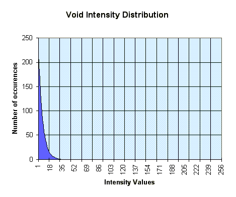
This prompted some statistical investigation into the nature of our data. Below, consider the four graphs which give the frequencies of the different codes in the hip.dat file. Notice how the void region has only one representative point. In the skin type, it becomes clear why changing the transparency settings for points in the range around 200 had such a noticeable effect. (incidentally, the 200 range corresponds roughly to the fourth control point, if all are spread equally along the range).

[On each graph, the reference counts have been normalized to the range 0-280 on the y axis; on the x axis, we have the range of values from 0-256, each corresponding to a particular intensity for that tissue type.]

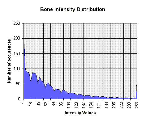
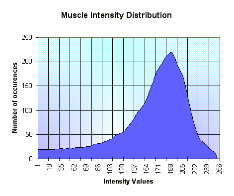
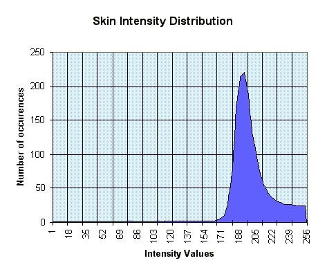
Notice that the spikes in the above graphs are very narrow. This makes it rather difficult for the user to specify, with reasonable accuracy, the transfer functions (the user would like to focus on the relevant areas : i.e. the spike itself, but there just isn't enough space for moving the control points inside the spike). Hence, we modified the transparency interface to automatically rescale the axes based on the frequency of the data. Additionally, we applied a weak smoothing algorithm to the frequency data and displayed the graphs on top of the normal parameter setting graphs.

The "rescaling" was done in the following manner :

we compute the integral of the distribution function as a simple Riemann sum

we then consider some sampling of the function along its domain and take the value of the function at those sample points.

the value of the function is adjusted as a percentage of the integral; this percentage is rounded then to the extent of the domain, giving the position of the point based on its weight.

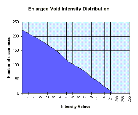
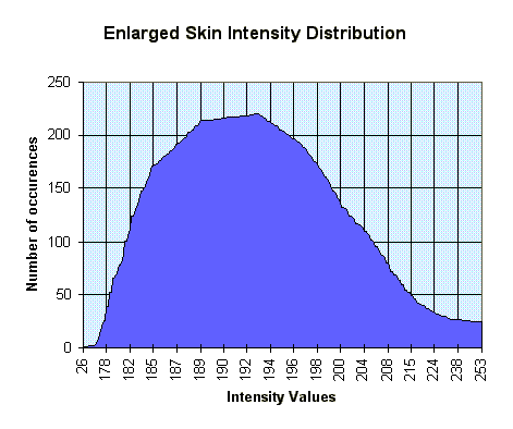
In this way, notice how points that are situated "beneath" high spikes in the function will spread out a lot because their respective percentages are very high and they will consequently take up a lot of real-estate on the function's domain.

[The graphs above & below are the enlarged versions of the above graphs, given the algorithm outlined. Notice the enlarging of x values on the X axis. Included are snapshots from the actual TCL interface].

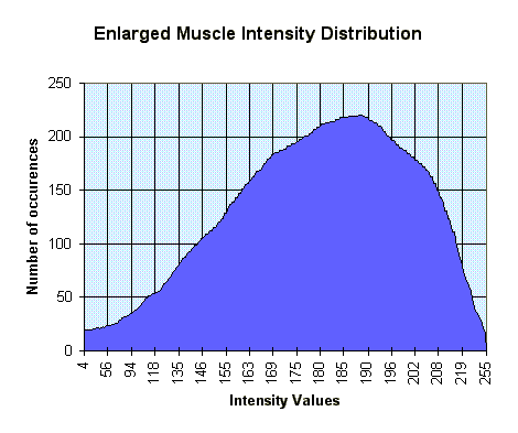
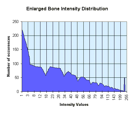
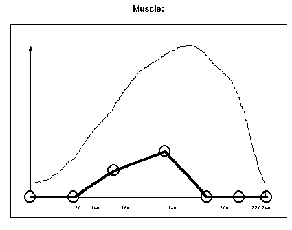
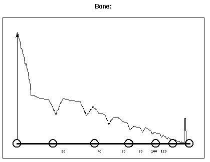
Although this lead to an interface that equalized the effect of each of the control points, the problem of spatial correlation still remains. Notice that making the skin a bit more transparent does not necessarily allow one to see that areas that they want.

Here are 2 images taken from the TCL interface :

the 'main' window

the 'transparencies selection' window

Future Development

The reason the TCL interface cannot provide the answers to all of our questions is because of spatial correlation problems. Although we have an idea where to move the points in order to get large changes in the transparency/intensity, we have no idea how these points are spread in the volume of the heap. For instance, the central bump in the structure of the muscle consists of points that come literally from everywhere in the hip; we'd have little if any control on localizing the transparency settings to particular areas in the hip or even generally in the image.
At this point, it seems that only by correlating the interface efforts with a design gallery search approach may we meet with success on this project.

The renderer has been engineered with save routines that produce graphics files that can be processed by the culling software written by Tom Kang & Josh Seims for their Design Gallery program.

In our state space search, the variable is the transfer function for the particular tissue types; at this early stage in the search development, we've simply chosen to vary the transfer function for the muscle by choosing 4 distinct positions on the Y axis, correlating the 7 control points in pairs of 2 (leaving 1 single) and varying them across the lattice. This produces 4⁵ = 1024 possibilities. The main obstacle we're hitting is that the space seems to be simply enormous : if we wish to have fine granularity in the way functions are specified, we ought to pick a relatively tight lattice for the graphs; this, conjectured with the fact that we have 7 control points and 4 graphs will create an inordinately large number of images. We have yet to figure out how to properly deal with this problem.

At present the TCL interface is fully functional (final touches recently added and gaps closed). In the future, once the Design Gallery will be implemented, the plan is to allow the user to choose an image that more or less satisfies their needs, recall the particular functional configuration for that image and then allow the user to fine tune it using the TCL interface (this may in fact be the key for reducing the number of images : we may allow the lattice to be somewhat rough because that will be compensated by fine tuning in the transfer function specifications).

To conclude, let me outline plans of future development :

1). Devise an efficient scheme for sampling the function space w/o creating a ridiculous number of images. Devise an algorithm/program for generating a tree structure on the space, once we've performed the culling. Design an appropriate interface for our particular Design Gallery implementation.

2). As a potential improvement, attempt to rotate the hip volume and save it back to disk for future use. This is underlined by the observation that it's unlikely the user will choose to change the viewpoint often, so it's advantageous to save a rotated volume and avoid all the rotation computations when rendering.