
The broadband Antenna Systems described here and on associated pages MAY NOT WORK FOR YOU ! They cannot operate well in every possible environment. Even with modifications and adjustments being identified and described and with very considerable extra effort there will be situations too difficult to manage.
This can be done from the Material Lists after consulting the System Drawing. It mainly consists of ordering finished PCBs, enclosures, cabling from the indicated sources.
After visual inspection of PCBs and other pieces Gasketing for the Preamp enclosure or Silicone rubber sealing needs to be completed. The ShackBoard needs to be assembled into the enclosure and front and rear panels attached. The top cover of the enclosure may be left off until later.
As of mid-February 2025 there is now an alternative to pouring a silicone rubber gasket. N3AGE has created an STL file for a gasket design that can be 3D printed and simply placed in the enclosure cover's channel. This has hast been proven with a gasket 3Dprinted at home and is a recommended simple replacement for the silicone and a significant time-saver for assembly. Apply dielectric grease on each side of the gasket prior to installing to insure a watertight seal. ]
Begin by applying Silicone Rubber to the channel in the enclosure cover using a wide spatula or painter's knife to create a gasket in the channel. Silicone rubber is preferred because it shrinks very little as it cures. This can be a little messy but clean up should be possible using mineral spirits if required. Don't worry about a little extra rubber where it was not intended but rather let it set for a few hours and come back to do clean up when it is partially set. Let it sit for a few DAYS to fully cure. Note that this enclosure should probably be considered "water resistant" rather than "water proof". Better designs are welcomed. FreeCad source code for the current design is provided. Below is a picture of a portion of the enclosure cover filled with gasket material.
Mount PCBs into their enclosures. The Preamp attaches with two brass 6-32 x 3/8" screws. The ShackBoard PCB slides into the extrusion and front and rear panels are attached with 3mm hardware that comes with the enclosure.
With both the Preamp and Shack Board PCBs complete and mounted, operation can be verified. Before applying power to the ShackBoard, measure across the barrel connector to be sure there is not a short. Then use a current limited or low current 12 VDC supply and verify that the green power LED lights. Total current should be limited to no more than 150 mA. Verify that the Bias Switch on the ShackBoard toggles lighting of the Blue LED near the rear of the board. Measure and set the LDO output voltage adjustment and verify that the output voltage varies as it is adjusted. Leave it at mid-range.
Verify that the ShackBoard is operating properly, whether the Utility or Performance option is being selected. With no CAT5 connecting the SAPreamp, measure the noise floor
Connect the Preamp to the ShackBoard with a standard, short CAT5 cable. On the Preamp verify the DC voltages shown in green on the schematic and indicated on the Preamp silkscreen.,Also verify that total current from the power supply is near 100 mA and that it changes when the Bias switch on the ShackBoard is toggled. Leave that switch and the dipole shorting switch in the enabled/On position toward the A side outputs of the ShackBoard.
Next connect the ShackBoard RF output to a spectrum analyzer or broad band SDR or even narrow band receiver. With total current verified to be in the vicinity of 100 mA, simply touching each of the antenna pads on the preamp with a finger one at a time should result in significant and similar change in output observed for each of the inputs.
If a difference is found, SMA connectors can be slipped onto the antenna pads, temporarily tack-soldered to the PCB . A TinyVNA can then be used to measure from that SMA connector to the ShackBoard A+ output to verify the swept response from 50 kHz to 200 MHz. It should look approximately the same as the SAS gain plot shown near the bottom of this page.Do that for both Preamp inputs is there is any doubt about operation.
When this PCB verification is successfully completed, .5mm diameter magnet wire, perhaps AWG #24 - #26, may be prepared in two lengths each a little bit longer than 3 meters. One end should be passed through the small entry hole in the PCB enclosure, tinned and soldered to its antenna pad for each monopole. There are two sets of pads on the newest design, one for Medium-Z and the other for high-Z optioning. Apply dielectric grease or other sealant on the inside of the entry holes to keep water from entering. When extended, the end enclosure screws may can be used as strain reliefs by passing the conductor around them. This also prevents water from flowing down the top conductor and into the hole. These conductors may be coiled pending attachment of the assembly to the fiberglass mast 3m below the top.
The mast is first extended to full length and plastic clips attached with TyWraps at the junction of each of the six upper sections. This placement further assures that a section can't collapse during use. Once the mast is complete with clips, the Preamp enclosure can be placed just below the third section, counting from the top, and the enclosure, cover and CAT5 cable placed in approximate position with the mast lying on the earth. Tywraps are then run through the cover and enclosure but left loose awhile CAT5 cable coupler is being connected to the RJ45 connector on the PCB using a very short run of CAT5 cable. That cable will be formed 90 degrees and set in the exit groove of the enclosure while the cover is fitted over the enclosure Prior to securing the cover some additional silicone rubber wll have benn used to seal the antenna wire and the CAT5 passage areas. The cover is secured with six more brass 6-32 screws into the tapped holes in the enclosure. Don't over-tighten these screws since the threads are in plastic and only require enough torque needed to snugly close the cover gasket onto the enclosure.
After the enclosure is sealed the CAT5 cable and individual monopole conductors are routed through the intermediate mast clips in both directions along the mast with the conductors tied off at the end clips around the arms. It's OK to wind a few turns of conductor aroundat the ends.
With the longer CAT5 cable in place, verify that total power supply current is the same and that the two LEDs on the Preamp's RJ45 are illuminated.
The question is "When?". As of the time of this writing, after many SAS deployments, failures have occurred. Other than a single production run of SAPreamp PCBs from JLCPCB which exhibited unconnected through-board via disconnects all other failures have been the result of water or moisture ingress into the SAPreamp enclosure. Unless extreme care is taken to keep the outdoor-mounted electronics inside the enclosure dry this will almost certainly be the cause of future failures in most climates. It is difficult to overstate the difficulty in keeping hardware exposed to the elements, having connecting cables and wires, from eventually leaking. The gasketing shown above is a requirement but even with that installed and performing well there are other paths for water into the preamp assembly. The worst of these may be by way of water from rain or condensation flowing down the upper monopole and into an imperfectly sealed upper access hole. The following picture shows a method currently used to mitigate this.
[picture of TyWrap routing of monopole conductors]
It is not yet certain how effective this method will be. Unless an installed preamp assembly can be completely immersed in water while staying dry inside, it seems that eventually water will enter and most likely destroy the preamplifier.
This failure mode is particularly a mechanical/environmental problem. The project is Open Source. It is hoped that other contributors will be able to modify the design in a way to make this type of failure far less likely.
If possible,prior to attaching the long CAT5 measure and record the insertion loss as a function of frequency. Knowing this will provide a better estimate antenna factor and e-field measurement and absolute signal and noise levels.
For reference, here are the standard CAT5 cable pairing connections used between the SAPreamp and the Shack Board RJ45 connectors and the pin connections used.
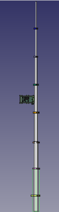
When complete, the High-Z SAS assembly should look like the picturebut with the addition of wire conductors and CAT5 cable and be ready for paint, if desired. Spraying everything with flat green or brown camouflage paint is not required but makes the finished system much less noticeable. This may be important in some HOA environments.
In general, the Single Antenna receive system can't be better than its location. While capable of rejecting unwanted noise and signal ingress from some common mechanisms such as poor symmetry, balance and feedline coupling, it won't be better than the near-field and far-field noise environment. Placed too close to local sources that generate fields producing high field gradient such that the tips of the dipole see different potentials, the system will convert these to differential signals which may raise the system noise floor and degrade SNR of propagated signals. Recognize that this ingress is different from "radiation" because it changes with distance in a very different manner compared to far-field, inverse-square, radiation. Small changes in position and polarization may provide a great deal of improvement in this respect. Keeping the mounting location well away from residences and sources of mains power, network signals is usually a good start. Mounting the dipole on or next to a building may be a bad choice. The SA has been designed to allow a nominal 100' length of CAT5 cable to be used. Taking advantage of as much physical separation as a site allows usually helps final results. To the extent possible, keep the antenna located at least one antenna height away from foliage and, particularly, other conductors such as antennas. See the discussion of scattering and shadowing for more detail about this.
Though CAT5 shielding is not essential, quality cable designed for outdoor or direct burial and using the largest conductor size and quality dielectric is important for practical reasons. As for the case with coaxial feedlines, keeping moisture away from the vicinity of the line is essential. At 30 MHz, 100' of the best quality CAT5 should have no more than 3dB attenuation. This has been compensated for in the SAPreamp design. When putting a system together the builder is advised to not only select a good product but also to stay aware of degradation due to water entering the region around the twisted pairs from nicks, abrasion or animal involvement. Not doing so can result in a degraded system and as for coaxial feedlines that process may not be immediately noticed.
The Field Probe, mentioned earlier, may be helpful in identifying
"quieter spots" in a candidate back yard or placement region.
Mounting close to buildings and other conductors is generally to be
avoided. Eliminating sources of unwanted signals may be an option
but is like playing "wack-a-mole" since new sources may always arise
later. It's better by far to site the SA well in the first place, to the
degree that is possible. Whether using a Field Probe or the SAS itself,
surveying a location for best final position can make a great deal of
difference in ultimate performance. A small change in location can often
make a very significant change in ultimate system noise floor and the SNR
delivered to the receiving system's detector.
At this point initial powered system testing may begin. With the mast vertical and bottom section either clamped to a short non-conductive post or else placed in the screw-in ground mount and freestanding, the CAT5 may be run to the Shack Board location and the entire system powered up for testing.
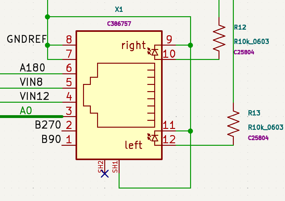
With mast, dipole, preamp, CAT5 cable and Shack Board installed and connected initial verification of the entire system can be performed. This step confirms that the common mode rejection capability of the system is being provided. This is most easily done through using the two switches on the Shack Board which are provided for that purpose.
Looking at a broad spectrum, either from a spectrum analyzer that covers at least 0-30 MHz or from an SDRs such as the KiwiSDR or WEB-888 which can provide the same display, simply observe that broadband display. Then, using the "Short the Dipole" switch on the Shack Board engage the mechanical relay at the dipole terminals. Confirm that ALL signals & noise being displayed drop in amplitude by 20 dB or more and that nothing near the previous level remains. Look for a very large drop in all responses. This test verifies that only differential signals from the antenna are significant and that common mode rejection of the system is being provided. When the MediumZ Performance option is being used, the other switch for buffer stage bias may be turned off which will extinguish the blue LED on the back panel.
Do not attempt to proceed until any signals and more importantly, their mechanism of ingress are identified and removed. Mechanisms that can produce these unwanted responses that would decrease system sensitivity by decreasing SNR of desired, propagated signals must be removed first. These important steps verifiy that "The antenna really is the antenna." Signals being produced are truly from the dipole acting as a differential source rather than from feedline, power supply, unbalance or some other form of unwanted ingress. This test can be periodically repeated to provide assurance that a system has not changed in this regard.
It's important to recognize that engaging the "Short the Dipole" switch DOES NOT remove signals from the Preamp input. It only assures that differential signals produced at the dipole center - across the mono-poles - are removed. Common mode signals will still appear between the Dipole, which has become a center-fed conductor, is still an antenna against the reference ground of the preamp. This 'ground' is the potential that exists at the end of the CAT5 cable. Because the entire system is now mono-pole with a horizontal element working against the CAT5 common potential, the Preamp and in particular the buffer input stages, are likely still dealing with large signals. This situation is depicted in the last graphic presented at the end of Whip_Tipps DL4ZAO (Google Translation). Shorting the monopole connections only assures that the differential signals from the dipole which is the desired antenna are dominant it doesn't eliminate common mode signals which may be present and perhaps even large enough to overload the preamplifier and cause unwanted distortion and generation of mixing products and a degraded system noise floor.
Even after the assurances provided by the verification methods it is possible that some unwanted signals may remain since near-field interference, local sources of unwanted signals and noise, can be converted to differential signals if and when the change in their fields across the length of the dipoles is sufficient to create a differential signal. This is to say, if the dipole lies along the gradient of very strong near-field sources the profile of the field strength versus distance will NOT follow an inverse square law as do propagated signals from very far away. Minimizing these unwanted sources becomes a major endeavor once the SAS is properly rejecting common mode ingress.
Since those near-field signals are, in a sense, "real" the first line of defense against them will be in changing antenna siting in either x, y or z directions slightly or perhaps even altering polarization to minimize the response in the system. If the source of a particular offending source is only quenched without changing antenna system siting then a susceptibility remains and may not be recognized when a another similar unwanted source arises. Ongoing vigilance is necessary to assure that a SAS is not responding to nearby unwanted interference that can restrict its overall performance.
It is important to understand that antenna size and component values within the SAPreamp and ShackBoards only provide a compromise between maximum sensitivity and avoidance of overload for typical amateur locations. This compromise will no doubt be less than perfect for any particular location. Arriving at the best choice of values becomes an ongoing effort. It may not ever be complete. A full-length 6m dipole is capable of achieving lower than ITU noise floor (noise temperature) values for a "Quiet Rural" location. This may be a considerably more difficult target than regional noise that common locations near residences, cities or such are capable of providing. This means that it may be possible to use a dipole that is shorter than 6m and not significantly degrade the resulting system. Analyzing this sort of change is a significant project but if it is found that there are extremely strong local signals anywhere in the 1 kHz - 200 MHz spectrum it could be that IMD within the Preamp or Shack Board will seriously degrade performance and a change will be required for best function.
If operation with the High-Z option cannot be obtained without significant antenna size reduction, the Medium-Z option may be chosen instead. This will sacrifice the LF performance but may be required to meet HF system. At sites that are also close to meeting the ITU Quiet Rural noise limits, this option may also be a best selection - though at the cost of VLF & LF operation. To operate in this option it will be necessary to modify the Preamp by removing the 0 ohm resistors from the high impedance buffer stages and to move the monopole connections to the Medium-Z pads indicated by the silkscreen.
After moving to this option, choose the largest dipole size possible that does not begin to exhibit overload as described above.
Along with the necessity to eliminate overload by component selection within the High-Z SA preamplifier and Shack Board hardware, it is also important to select best antenna size and to optimize weak signal reception. This is an issue of optimizing an entire receive system to be able to detect and demodulate signals down to the propagated noise level at the antenna. It is why the measured ITU noise levels have been selected as goals for system design. Not every location has the same limitations or potential. Some very good locations may bepotentially achieve the ITU "Quiet Rural" levels. For an omnidirectional antenna system, this is approximately the best that can be done anywhere in the world. If a particular locations ultimate ITU level is higher than this there is no benefit in outfitting it with an antenna system that can potentially do better. There may be practical benefit in NOT using such a capable system since dipole antenna size might be reduced with no degradation in performance while at the same time a smaller dipole might have more ability to tolerate very large signals. Up to about a half wavelength in size larger antennas generally have larger signal levels at their terminals, so deploying a less sensitive system may have overall benefits.
Because of this need for it is particularly important to make an initial assessment of any proposed site prior to deployment in order to best select antenna size and perhapscomponent values to give the greatest likelihood of providing the best strong-signal protection while simultaneously providing the highest system sensitivity. The topics below are intended to deploy a broadband receive-only antenna system kit and, once deployed, to optimize its performance for a specific location.
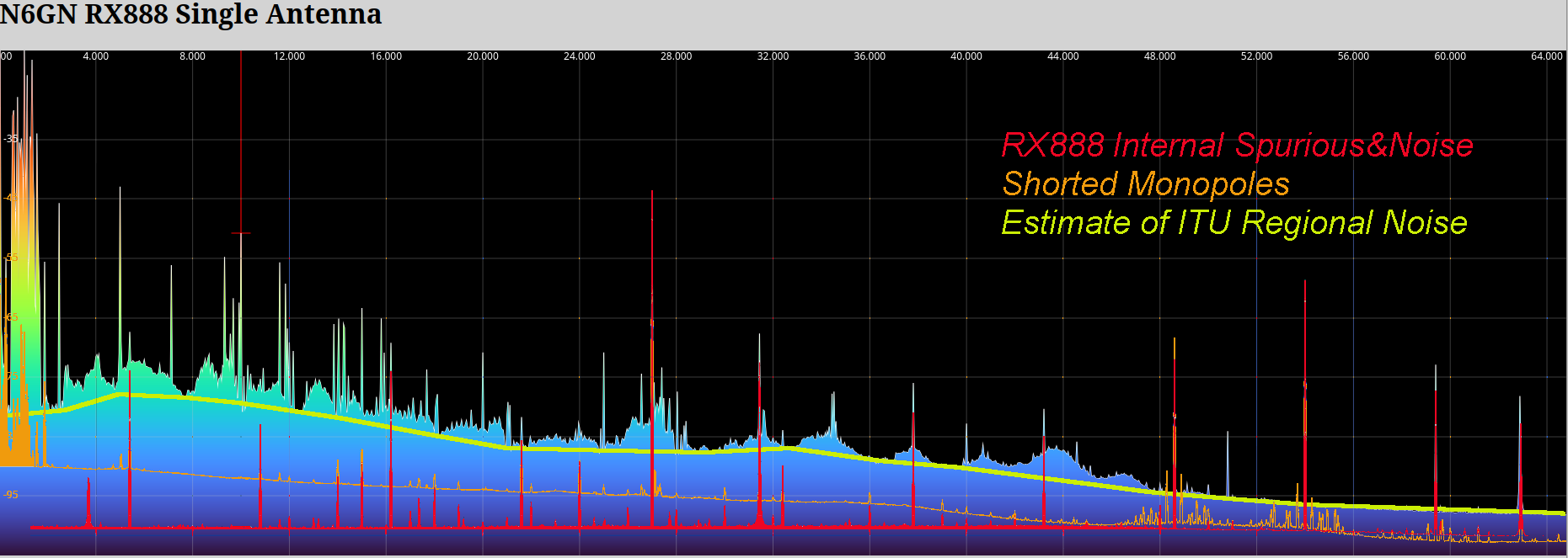
Four ITU Regional noise curves are used to evaluate the noise floor of an SAS. They are "City", "Residential", "Quiet" and "Quiet Rural". These regions are not precisely defined by the ITU. They describe a range of values taken over a large number of locations, seasons and solar conditions worldwide. Quiet Rural describes a minimum level for propagated manmade noise when the ionosphere is involved.
The Preamp output noise plot (in dotted red) from the QUCS model can be compared with ITU median regional noise levels. This shows that this configuration does not quite achieve the Quiet Rural limit. An alternate configuration which bypasses the input buffers is capable of superior noise performance that can equal or exceed the Quiet Rural requirements but at the loss of ELF/VLF operation.
Additionally, if at a particular deployment location, there are very large signals present that cause distortion then after verifying that the distortion is produced within the SA system rather than in a SDR that follows, antenna size or Preamp PCB component values may have to be changed to provide protection from this type of overload. These changes could increase the SAS noise floor and system temperature making it incapable of performing at the limit shown. Optimization is a process of finding a compromise between unwanted distortion and noise products and minimum noise floor, that is to say, maximum sensitivity and dynamic range.
Before changes are made it is important to determine the source of distortion, whether it is within the SAS or the SDR which follows. This is most easily done by inserting 10 dB or so of extra attenuation beween them. If there is no change and the evidence persists then the SA Preamp needs to be adjusted. After the SDR has been protected in this way so that it does not become the source of distortion, the SAS can be examined.
The following plot is from an RX888 being displayed by ka9q-web to demonstrate some of the limitations to the system sensitivity. It is taken from a small residential community with regional noise that is likely near ITU "Residential" .
See "Antenna Factor" below for more detail.
It may be useful to consider what is being attempted and what work may remain.
Each of the above items may change at any time. Because perfection has not been achieved, there are likely items which could benefit from further attention. There are many factors affecting maintaining or improving the overall performance which need to be monitored and verified.
The 6m dipole size and accompanying preamp has been targeted to create a system capable of achieving ITU Quiet Rural performance in the best of regions while simultaneously offering extremely broadband operation. It doesn't quite achieve this goal. Modifications to meet the requirements of particular locales are possible. Dipole length, conductor diameter, height and polarization may all be varied. However, the interactions among these variables are complex. It is to be expected that making the dipole either longer or using larger conductor diameter will not create a better result. But in some circumstances making the dipole shorter may prove to give a net improvement in terms of visibility and strong signal handling. This may result in no loss of performance in locales that don't meet the Quiet Rural level since even though the Single Antenna system noise floor may increase it may still remain below that of the region. For environments with extremely strong local signals that overload the input buffer stages, it is possible to entirely bypass the buffer stage and drive the ADA4930 CAT5 driver directly. This achieves significantly greater strong signal tolerance at the cost of loss of ELF/VLF noise floor.
Increasing the diameter of the conductor should similarly produce no significant improvement and may unbalance the antenna. The approximately .5mm diameter was chose as a compromise between low interaction with the CAT5 feedline cable and the ability to survive wind and ice loading. Because the preamp is a high impedance device, very little current flows in the dipole conductor so there is very little loss that larger conductor diameter might noticeably reduce.
Polarization can be varied. Vertical polarization was chosen to provide the lowest practical beam for long distance ionospheric propagation but rotating the dipole horizontally may reduce noise while increase ground absorption and take-off angle. This may be a good solution for NVIS propagation in those portions of the spectrum where it is possible. Rotating toward horizontal polarization may also add some flexibility in rejecting strong nearby vertically polarized MW broadcast transmitters that could otherwise drive buffer stages into overload and make the entire assembly unusable.
Mounting location is a significant variable. Particularly in locations limited by unwanted local noise sources, moving the antenna horizontally or vertically may have a dramatic effect on delivered SNR. It may be that a shorter dipole moved upward can still potentially deliver the regional ITU noise performance by reducing coupling to local near field noise. But moving vertically may also increase the level of strong signals present at the preamp input so risks the system entering into overload. As an example, a 3m dipole at the top of a 10m mast may deliver better SNR than a 6m dipole at minimum height on a 7m mast while also having better immunity to overload.
Generally speaking as applied this is a low Q non-resonant antenna. No single parameter is sensitive or has a large effect on performance. Reducing the length by a factor of two can be expected to reduce signal level > 6 dB where the antenna is electrically short since the recovered voltage is reduced by two. At shorter wavelengths where the dipole is a half-wave or longer the maximum signal level will increase only slightly even at very large electrical size while the pattern will vary wildly. This too is a possible means of mitigate strong unwanted local VHF signals.
Modifications of this system may greatly improve the performance but interactions among the variables must be studied and controlled to achieve maximum benefit from any change. The overall environment may change in a multitude of ways so constant monitoring and verification, comparison of performance with other stations and general observation are necessary to maintain the best performance.